Question: In Microsoft Excel 2013, I've created a pivot table with two fields in the Values Section of the pivot table. These fields are the sum of the Quantity as well as the sum of the Total cost of an order. The pivot table seems to be populating the Values section in multiple columns and I want to see the results in a single column.
How can I set up my pivot table so that the Quantity and Total cost (in the Values section) values show up in a single column instead of being listed in two?
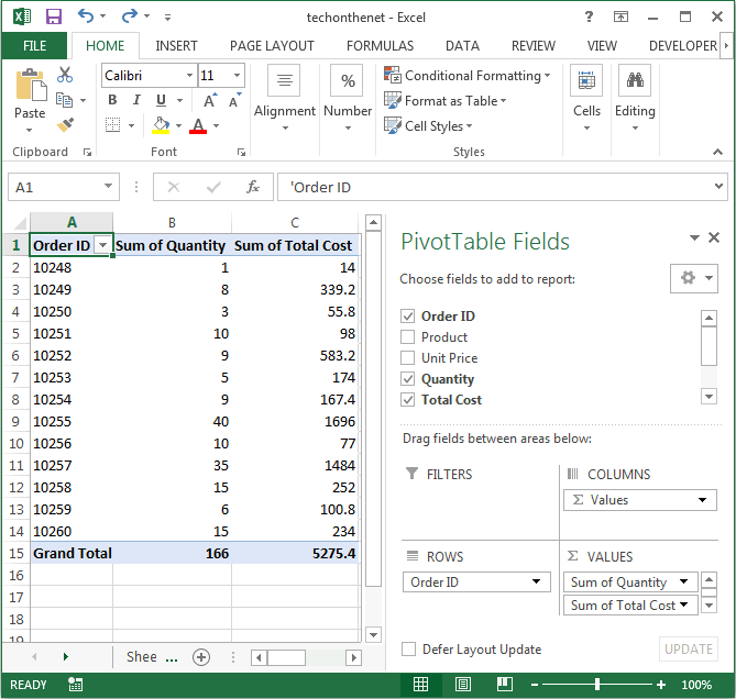
Answer: Excel may format your Values section of your pivot table to populate your values in multiple columns. In this example, you can see that the "Sum of Quantity" as well as "Sum of Total Cost" fields are being displayed in multiple columns. We want to see these values in a single column.

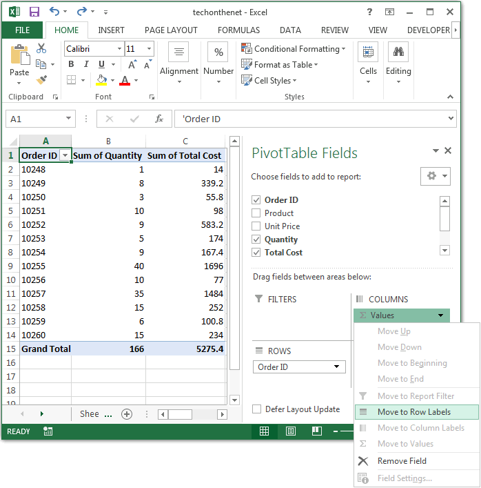
Under the COLUMN section, right click on the Values field and select Move Values to Row Labels from the popup menu.

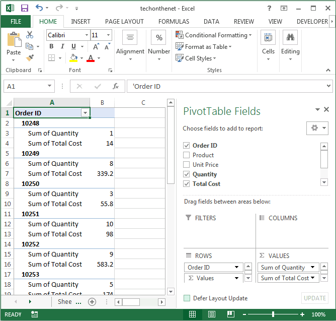
Now your pivot table should display the "Sum of Quantity" and "Sum of Total Cost" fields in a single column, populating down.
