Question: How do I display a hidden value in a pivot table in Microsoft Excel 2013?
Answer: To explain how to display a hidden value in an Excel pivot table, we'll take a look at an example. In this case, the entry for Order ID 10249 is hidden.

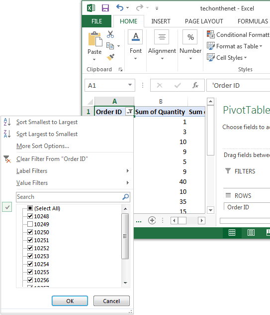
Click on the arrow to the right of the field that has the hidden value. In this example, the field that has the hidden value is called Order ID, so we'll click on the arrow to the right of the Order ID field.

Check the box to the left of the value that you want to display. Click on the OK button. In this example, we want to check the box for Order ID 10249.
Just to summarize, all checked values are visible in the pivot table and all unchecked values are hidden in the pivot table.

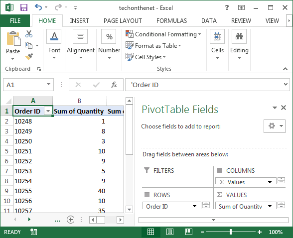
Now when we return to the pivot table, we can see the details for Order ID 10249.